Read spatial omics

[1]:

import SOAPy_st as sp
import pandas as pd

Read Visium

we used 10X Visium data of mouse dorsolateral prefrontal cortex (DLPFC, 151676) as an example to read the 10X Visium data. To prepare raw data, follow these steps:

1.Raw data file could be download from https://research.libd.org/globus/.

2.Click jhpce#HumanPilot10x and 151676 in turn.

3.Download 151676_raw_feature_bc_matrix.h5, tissue_hires_image.png, tissue_lowres_image.png, tissue_positions_list.txt and scalefactors_json.json.

4.Rename tissue_positions_list.txt to tissue_positions_list.csv.

5.Assemble the folders as 151676/151676_raw_feature_bc_matrix.h5 , 151676/spatial/tissue_hires_image.png, 151676/spatial/tissue_lowres_image.png, 151676/spatial/tissue_positions_list.csv and 151676/spatial/scalefactors_json.json.

[2]:

adata_visium = sp.pp.read_visium2adata(
    path = './151676/',
    count_file = '151676_raw_feature_bc_matrix.h5'
)

/home/wangheqi/anaconda3/envs/SpatialOmics/lib/python3.9/site-packages/anndata/_core/anndata.py:1832: UserWarning: Variable names are not unique. To make them unique, call `.var_names_make_unique`.
  utils.warn_names_duplicates("var")

[3]:

adata_visium

[3]:

AnnData object with n_obs × n_vars = 4992 × 33538
    obs: 'in_tissue', 'array_row', 'array_col'
    var: 'gene_ids', 'feature_types', 'genome'
    uns: 'spatial'
    obsm: 'spatial'

Read GeoMx DSP

Read spatial transcriptomics data of NanoString GeoMx DSP. Mouse embryonic development samples are used as examples.

Download Count Results and E13 Images files from https://nanostring.com/products/geomx-digital-spatial-profiler/spatial-organ-atlas/mouse-development/ .

[4]:

adata_dsp = sp.pp.read_dsp2adata(
    # The path of 'Images' files
    xml_file={
        # Using the xml file for two samples as an example,
        # you can add key-value pairs to the dictionary if you need information about sample points for more samples.
        'mu_dev_E13_006': './nanostring_growth/mu_dev_E13_006.ome.xml',
        'mu_dev_E13_011': './nanostring_growth/mu_dev_E13_011.ome.xml'
    },
    # The path of Count Results
    information_file='./nanostring_growth/Export4_NormalizationQ3.xlsx',
)

[5]:

adata_dsp.obs.head()

[5]:

	SlideName	ScanLabel	ROILabel	SegmentLabel	QCFlags	AOISurfaceArea	AOINucleiCount	ROICoordinateX	ROICoordinateY	RawReads	...	Timepoint	ROIID	SegmentID	ScanWidth	ScanHeight	ScanOffsetX	ScanOffsetY	LOQ (Mouse NGS Whole Transcriptome Atlas RNA)	NormalizationFactor	ExpressionFilteringThreshold (Mouse NGS Whole Transcriptome Atlas RNA)
SegmentDisplayName
mu_dev_E9_001 \| 001 \| Full ROI	mu_dev_E9_001	mu_dev_E9_001	1	Full ROI	Low Negative Probe Count for Probe Kit Mouse N...	47287.021916	392	16573	18896	4259786	...	E9	c73163bc-f107-498f-bd40-bbcab9a48993	f057dc6e-68ce-441d-a816-58802fc38258	16904.210938	20578.818359	7932	6094	16.252453	0.536152	16.252453
mu_dev_E9_001 \| 002 \| Full ROI	mu_dev_E9_001	mu_dev_E9_001	2	Full ROI	Low Negative Probe Count for Probe Kit Mouse N...	41175.373907	340	16485	19752	4725639	...	E9	be667b65-38c0-49c4-af51-845ffd8a7a85	09985ba0-449c-4b1a-9c8f-9327991df8fa	16904.210938	20578.818359	7932	6094	17.745085	0.496225	17.745085
mu_dev_E9_001 \| 003 \| Full ROI	mu_dev_E9_001	mu_dev_E9_001	3	Full ROI	Low Negative Probe Count for Probe Kit Mouse N...	43198.870210	403	15756	18824	5958816	...	E9	ba522e1c-7e21-4cc6-b529-118603949d5a	2ac08d0d-c65d-4ab9-b834-5ef7ebbad4cd	16904.210938	20578.818359	7932	6094	18.109046	0.395298	18.109046
mu_dev_E9_001 \| 004 \| Full ROI	mu_dev_E9_001	mu_dev_E9_001	4	Full ROI	Low Negative Probe Count for Probe Kit Mouse N...	44444.810459	368	15722	19675	3703922	...	E9	52d9a6b1-934d-4f42-a80e-a4a78b7ede43	aeed549d-8b7a-4fa4-b22a-c54059e83066	16904.210938	20578.818359	7932	6094	14.509348	0.605782	14.509348
mu_dev_E9_001 \| 005 \| Full ROI	mu_dev_E9_001	mu_dev_E9_001	5	Full ROI	Low Negative Probe Count for Probe Kit Mouse N...	31889.529594	279	15064	18429	3069897	...	E9	a9e0bca3-59a4-4131-90b7-c787ca400759	c53d1b52-712e-4a3d-9af4-5bdb55365eef	16904.210938	20578.818359	7932	6094	12.118616	0.717618	12.118616

5 rows × 35 columns

The sampling points corresponding to each ROI is stored in.uns.point.

[6]:

adata_dsp.uns['point']

[6]:

	slide	roi	x	y
0	mu_dev_E13_006	1	13011.793535	10484.417086
1	mu_dev_E13_006	1	13109.708338	10499.139178
2	mu_dev_E13_006	1	13184.708338	10547.123928
3	mu_dev_E13_006	1	13242.708338	10642.093747
4	mu_dev_E13_006	1	13261.840745	10730.656697
...	...	...	...	...
4171	mu_dev_E13_011	58	4548.893838	10387.159712
4172	mu_dev_E13_011	58	4477.882657	10362.799483
4173	mu_dev_E13_011	58	4437.660936	10371.299021
4174	mu_dev_E13_011	58	4487.202775	10425.060315
4175	mu_dev_E13_011	58	4636.188087	10423.920083

4176 rows × 4 columns

Read other barcode-based data

In most cases, the raw data of barcode-based spatial omics technology can be expressed in two tables: the coordinate information of each cell (spot) and the expression of each cell (spot). This sp.pp.read_csv2adata() generates the Anndata format by providing the two tables by the user.

Here we use slide-seqV2 data from the mouse olfactory bulb as a demonstration. Download Puck_200127_15.digital_expression.txt.gz and Puck_200127_15_bead_locations.csv from https://singlecell.broadinstitute.org/single_cell/study/SCP815.

[7]:

express = pd.read_csv('./Slide_seqV2/Puck_200127_15.digital_expression.txt', index_col=0, header=0, sep='\t')
location = pd.read_csv('./Slide_seqV2/Puck_200127_15_bead_locations.csv', index_col=0, header=0)

[8]:

adata_csv = sp.pp.read_csv2adata(express.T, spatial=location)

[9]:

adata_csv

[9]:

AnnData object with n_obs × n_vars = 21724 × 21220

Read imaged-based data

The image-based spatial omics technology needs to perform cell segmentation first, and quantitatively generate anndata format through the results of cell segmentation. Users are required to provide images of cell segmentation and staining images for each marker.

Here we use one (sample 1) of breast cancer MIBI-TOF dataests as an example. Download from https://mibi-share.ionpath.com. chick Ji, Rubin, Thrane, Jiang et al.’s Download.

[10]:

import tifffile as tiff
import matplotlib.pyplot as plt
import cv2 as cv
image = tiff.imread('./mibi_tof/TA459_multipleCores2_Run-4_Point1.tiff')
mask = cv.imread('./mibi_tof/TA459_multipleCores2_Run-4_Point1/segmentation_interior.png')
mask = mask[:, :, 0]

[11]:

plt.imshow(mask, cmap='gray')
plt.show()

../_images/Tutorials_Read_spatial_omics_20_0.png

[12]:

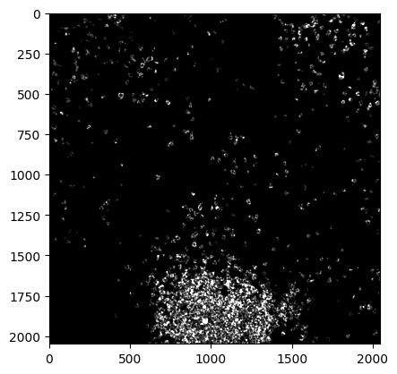
plt.imshow(image[8, :, :], cmap='gray', vmax=5)
plt.show()

../_images/Tutorials_Read_spatial_omics_21_0.png

Determine the name of each channel and the channel that needs to be removed to obtain the quantitative Anndata.

[13]:

channel_names=[
    'Au','Background','Beta_catenin','Ca','CD11b','CD11c','CD138','CD16','CD20','CD209','CD3',
    'CD31','CD4','CD45','CD45RO','CD56','CD63','CD68','CD8','dsDNA','EGFR','Fe','FoxP3','H3K27me3',
    'H3K9ac','HLA-DR','HLA-I','IDO','CK17','CK6','Ki67','Lag3','MPO','Na','P','p53','PanCK','PD-L1',
    'PD-1','pS6','Si','SMA','Ta','Vimentin'
]

exp_removed = [0,1,3,19,21,23,33,34,40,42]

[14]:

adata_img = sp.pp.read_mult_image2adata(
    image=image,
    mask=mask,
    channel_names=channel_names,
    remove_channels=exp_removed
)

[15]:

adata_img

[15]:

AnnData object with n_obs × n_vars = 5240 × 44
    uns: 'img', 'mask', 'var_for_analysis', 'spatial', 'SOAPy'
    obsm: 'spatial'